How To Create A Forecast Sheet In Excel

Many of us fell in love with Excel as we delved into its deep and sophisticated formula features. Because there are multiple ways to get results, you can decide which method works best for you. For example, there are several ways to enter formulas and calculate numbers in Excel.

5 ways to enter formulas

1. Manually enter Excel formulas:

Long Lists: =SUM(B4:B13)

Short Lists: =SUM(B4,B5,B6,B7) or=SUM(B4+B5+B6+B7). Or, place your cursor in the first empty cell at the bottom of your list (or any cell, really) and press the + sign, then click B4; press the plus sign again and click B5; and so on to the end; then press Enter. Excel adds up this list you just "pointed to" as =+B4+B5+B6+B7.

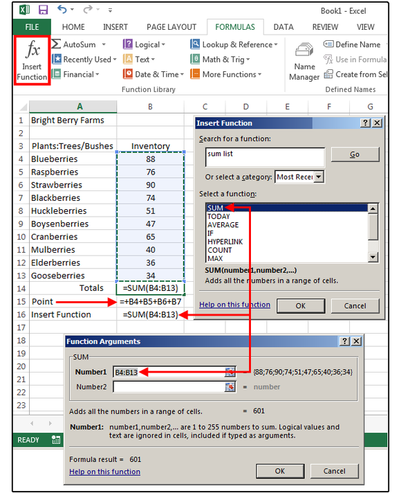
2. Click the Insert Function button

Use the Insert Function button under the Formulas tab to select a function from Excel's menu list:

=COUNT(B4:B13) Counts the numbers in a range (ignores blank/empty cells).

=COUNTA(B3:B13) Counts all characters in a range (also ignores blank/empty cells).

3. Select a function from a group (Formulas tab)

Narrow your search a bit and choose a formula subset for Financial, Logical, or Date/Time, for example.

=TODAY() Inserts today's date.

4. The Recently Used button

Click the Recently Used button to show functions you've used recently. It's a welcome timesaver, especially when wrestling with an extra-hairy spreadsheet.

=AVERAGE(B4:B13) adds the list, divides by the number of values, then provides the average.

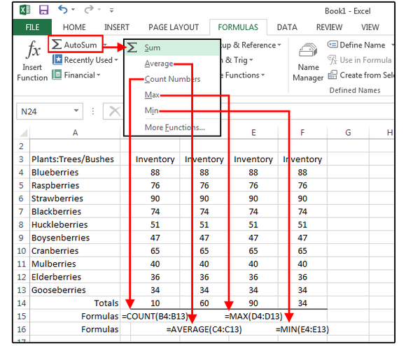
5. Auto functions under the AutoSum button

Auto functions are my editor's personal favorite, because they're so fast. Select a cell range and a function, and your result appears with no muss or fuss. Here are a few examples:

=MAX(B4:B13) returns the highest value in the list.

=MIN(B4:B13) returns the lowest value in the list.

AutoSum in Excel — Use the AutoSum button to calculate basic formulas such as SUM, AVERAGE, COUNT, etc.

Note: If your cursor is positioned in the empty cell just below your range of numbers, Excel determines that this is the range you want to calculate and automatically highlights the range, or enters the range cell addresses in the corresponding dialog boxes.

Bonus tip: With basic formulas, the AutoSum button is the top choice. It's faster to click AutoSum>SUM (notice that Excel highlights the range for you) and press Enter.

Another bonus tip: The quickest way to add/total a list of numbers is to position your cursor at the bottom of the list and press Alt+ = (press the Alt key and hold, press the equal sign, release both keys), then press Enter. Excel highlights the range and totals the column.

12 handy formulas for common tasks

The five formulas below may have somewhat inscrutable names, but their functions save time and data entry on a daily basis.

Note: Some formulas require you to input the single cell or range address of the values or text you want calculated. When Excel displays the various cell/range dialog boxes, you can either manually enter the cell/range address, or cursor and point to it. Pointing means you click the field box first, then click the corresponding cell over in the worksheet. Repeat this process for formulas that calculate a range of cells (e.g., beginning date, ending date, etc.)

1. =DAYS

This is a handy formula to calculate the number of days between two dates (so there's no worries about how many days are in each month of the range).

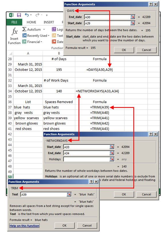
Example: End Date October 12, 2015 minus Start Date March 31, 2015 = 195 days

Formula: =DAYS(A30,A29)

2. =NETWORKDAYS

This similar formula calculates the number of workdays (i.e., a five-day workweek) within a specified timeframe. It also includes an option to subtract the holidays from the total, but this must be entered as a range of dates.

Example: Start Date March 31, 2015 minus End Date October 12, 2015 = 140 days

Formula: =NETWORKDAYS(A33,A34)

3. =TRIM

TRIM is a lifesaver if you're always importing or pasting text into Excel (such as from a database, website, word processing software, or other text-based program). So often, the imported text is filled with extra spaces scattered throughout the list. TRIM removes the extra spaces in seconds. In this case, just enter the formula once, then copy it down to the end of the list.

Example: =TRIM plus the cell address inside parenthesis.

Formula: =TRIM(A39)

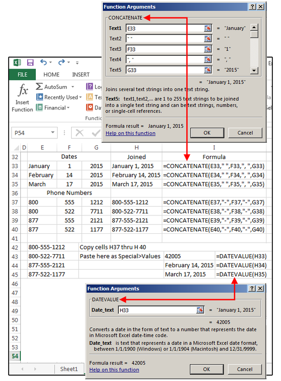
4. =CONCATENATE

This is another keeper if you import a lot of data into Excel. This formula joins (or merges) the contents of two or more fields/cells into one. For example: In databases; dates, times, phone numbers, and other multiple data records are often entered in separate fields, which is a real inconvenience. To add spaces between words or punctuation between fields, just surround this data with quotation marks.

Example: =CONCATENATE plus (month,"space",day,"comma space",year) where month, day, and year are cell addresses and the info inside the quotation marks is actually a space and a comma.

Formula: For dates enter: =CONCATENATE(E33," ",F33,", ",G33)

Formula: For phone numbers enter: =CONCATENATE(E37,"-",F37,"-",G37)

5. =DATEVALUE

DATEVALUE converts the above formula into an Excel date, which is necessary if you plan to use this date for calculations. This one is easy: Select DATEVALUE from the formula list. Click the Date_Text field in the dialog box, click the corresponding cell on the spreadsheet, then click OK, and copy down. The results are Excel serial numbers, so you must choose Format>Format Cells>Number>Date, and then select a format from the list.

Formula: =DATEVALUE(H33)

6. =FORMULATEXT

Use this function to display the "text" of a formula in a given cell. For example, the actual formula in cell E2 is =SUM(C2*D2); but all you see is the answer, which is $164.25. Sometimes it's helpful, even necessary, to see the actual function, especially if you're editing a macro or tracking down a circular reference. So enter this formula into a cell off to the side of your spreadsheet matrix (such as cell F2): =FORMULATEXT(E2) and Excel displays the actual formula of E2.

7. =AVERAGE

Averages are used every day to determine the median or midpoint of a set of numbers; for example, average grades for a group of students; average temperature of a region; and/or average height of sixth graders. Before functions, to get an average, you would add a column of numbers; for example 10 numbers; then divide by that total (10). The AVERAGE function does that for you. So typing =AVERAGE(E2:E6) adds those five numbers, then divides by 6.

8. =COUNT & =COUNTA

These simple functions count the total number of digits or text in a column of data. COUNT only counts numbers and formulas, while COUNTA counts everything—that is, alpha and numeric characters plus punctuation, symbols, and even spaces.

Why use the COUNT function? Imagine that your friends pay dues for membership into several different clubs. The spreadsheet adds the dues for all clubs in column G, so each individual knows how much he/she owes in dues a month. Use the COUNT function to total the number of people in each club (without having to create a column full of ones). For example; =COUNT(B12:B21) tells us there are six people in the Garden Club.

9. =COUNTBLANK

The COUNTBLANK function does exactly what is says: It counts the number of blank cells in a column or range. In column B of our spreadsheet example, there are four blank cells (and six cells with numbers). Note that anything in a cell, even a space, will register as a non-blank cell. In other words, if you put a space in cell B13, the total blank cells changes from 4 to 3.

10. =COUNTIF & combined functions

This formula combines the COUNT and the IF functions to count the number of cells in a range that meet a specific condition.

For example, say that you want to count the number of members in the Music Club (column C), but only the members who receive the discounted price of $18.00 a month. First you count the cells, then set the condition; for example: =COUNTIF(C13:C22, "<19"). In this case, the answer is 2. Note: Don't forget to put the conditions inside double quotes, or else you'll receive an error.

You can also combine multiple functions to get the results you need, so you don't have to use multiple cells or columns, which wastes valuable spreadsheet real estate. For example, imagine that you need to know how many cells are in a column or range with numbers (or text) plus the blanks.

For the numbers plus the blanks, enter this formula:

=COUNT(B13:B22) + COUNTBLANK(B13:B22)

For all characters (alpha and numeric) plus the blanks, enter this formula:

=COUNTA(B13:B22) + COUNTBLANK(B13:B22)

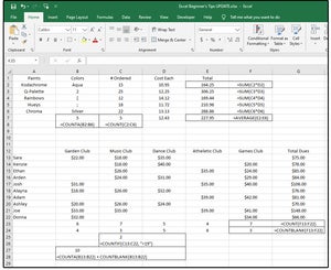
new checkout the average formulatext and four count functions — Checkout the Average, FormulaText, and four Count functions

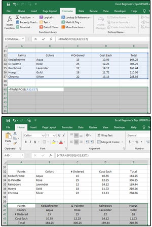
11. =TRANSPOSE

A very useful function if you decide to change the spreadsheet fields (columns) to rows and vice versa. Why would anyone do this? Sometimes when spreadsheets are created, we aren't absolutely certain which data should be the fields and which should be the records and, sometimes, the situation changes and requires a redesign. This is where the Transpose function comes in.

First, select a range of blank cells beneath (or on another sheet) that's the same size as the original range. Note that the original number of columns/fields may be five, while the rows/records are six. When you transpose the data, you'll have six columns and five rows; so be sure your blank cells reflect that. The original range may be A32:E37, but the new range of blank cells highlighted should be A40:E44.

Once the new range is highlighted, type =TRANSPOSE(A32:E37) in the highlighted section and use the original range coordinates. Once the function and range are entered, press Ctrl+Shift-Enter. and the range changes right before your eyes.

12. =MAX & =MIN

These two are simple, but useful. If you need to find the maximum or minimum number of items in a column or list, position your cursor somewhere outside the matrix and enter this function for Maximum: =MAX(E33:E37) or this for the Minimum: =MIN(D33:D37). Excel returns the highest or lowest number in the column list.

new try the transpose min and max functions — Try the Transpose, Min, and Max functions

Three more formula tips

As you work with formulas more, keep these bonus tips in mind to avoid confusion:

Tip 1: You don't need another formula to convert formulas to text or numbers. Just copy the range of formulas and then paste as Special>Values. Why bother to convert the formulas to values? Because you can't move or manipulate the data until it's converted. Those cells may look like phone numbers, but they're actually formulas, which cannot be edited as numbers or text.

Tip 2: If you use Copy and Paste > Special > Values for dates, the result will be text and cannot be converted to a real date. Dates require the DATEVALUE formula to function as actual dates.

Tip 3: Formulas are always displayed in uppercase; however, if you type them in lowercase, Excel converts them to uppercase. Also notice there are no spaces in formulas. If your formula fails, check for spaces and remove them.